Hi, everyone!
Blogspot has been a great platform for me, but in the end, editing posts with source code and mathematics has been too much of a headache in the neglected blogspot and google UIs.
Elsewhere in the universe, WordPress has developed and encouraged a great ecosystem of plugins that let you do LaTeX and code syntax highlighting directly in your posts with ease. I can't spend hours and hours on fixing mangled posts. It's time to move on.
So as of today, I am moving to a self-hosted blog at http://MathCancer.org/blog/
I will leave old posts here and gradually migrate them over to MathCancer.org/blog. Thanks for following me over the last few years.

Wednesday, August 10, 2016
Wednesday, February 24, 2016
Saving MultiCellDS data from BioFVM
Note: This is the fifth in a series of "how-to" blog posts to help new users and developers of BioFVM.
A BioFVM MultiCellDS digital snapshot includes program and user metadata (more information to be included in a forthcoming publication), an output of the microenvironment, and any cells that are secreting or uptaking substrates.
As of Version 1.1.0, BioFVM supports output saved to MultiCellDS XML files. Each download also includes a matlab function for importing MultiCellDS snapshots saved by BioFVM programs. This tutorial will get you going.
BioFVM (finite volume method for biological problems) is an open source code for solving 3-D diffusion of 1 or more substrates. It was recently published as open access in Bioinformatics here:
http://dx.doi.org/10.1093/bioinformatics/btv730
The project website is at http://BioFVM.MathCancer.org, and downloads are at
http://BioFVM.sf.net.
BioFVM*.cpp and BioFVM*.h (from the main BioFVM directory)
pugixml.* (from the main BioFVM directory)
Makefile and MultiCellDS_test.cpp (from the examples directory)
Open the MultiCellDS_test.cpp file to see the syntax as you read the rest of this post.
See earlier tutorials (below) if you have troubles with this.
// the program name, version, and project website:
BioFVM_metadata.program.program_name = "BioFVM MultiCellDS Test";
BioFVM_metadata.program.program_version = "1.0";
BioFVM_metadata.program.program_URL
= "http://BioFVM.MathCancer.org";
// who created the program (if known)
BioFVM_metadata.program.creator.surname = "Macklin";
BioFVM_metadata.program.creator.given_names = "Paul";
BioFVM_metadata.program.creator.email = "Paul.Macklin@usc.edu";
BioFVM_metadata.program.creator.URL
= "http://BioFVM.MathCancer.org";
BioFVM_metadata.program.creator.organization
= "University of Southern California";
BioFVM_metadata.program.creator.department
= "Center for Applied Molecular Medicine";
BioFVM_metadata.program.creator.ORCID = "0000-0002-9925-0151";
// (generally peer-reviewed) citation information for the program
BioFVM_metadata.program.citation.PMID = "26656933";
BioFVM_metadata.program.citation.PMCID = "PMC1234567";
BioFVM_metadata.program.citation.text
= "A. Ghaffarizaeh, S.H. Friedman, and P. Macklin, BioFVM: an efficient parallelized diffusive transport solver for 3-D biological simulations, Bioinformatics, 2015. DOI: 10.1093/bioinformatics/btv730.";
BioFVM_metadata.program.citation.notes = "notes here";
BioFVM_metadata.program.citation.URL
= "http://dx.doi.org/10.1093/bioinformatics/btv730";
// user information: who ran the program
BioFVM_metadata.data_citation.PMID = "12345678";
BioFVM_metadata.data_citation.PMCID = "PMC1234567";
BioFVM_metadata.data_citation.text
= "A. Ghaffarizaeh, S.H. Friedman, and P. Macklin, BioFVM: an efficient parallelized diffusive transport solver for 3-D biological simulations, Bioinformatics, 2015. DOI: 10.1093/bioinformatics/btv730.";
BioFVM_metadata.data_citation.notes = "notes here";
BioFVM_metadata.data_citation.URL
= "http://dx.doi.org/10.1093/bioinformatics/btv730";
set_save_biofvm_mesh_as_matlab( false );
Similarly, BioFVM defaults to saving the values of the substrates in a compact Level 3 matlab file. You can override this with:
set_save_biofvm_data_as_matlab( false );
BioFVM by default saves the cell-centered sources and sinks. These take a lot of time to parse because they require very hierarchical data structures. You can disable saving the cells (basic_agents) via:
set_save_biofvm_cell_data( false );
Lastly, when you do save the cells, we default to a customized, minimal matlab format. You can revert to a more standard (but much larger) XML format with:
set_save_biofvm_cell_data_as_custom_matlab( false );
save_BioFVM_to_MultiCellDS_xml_pugi( "sample" , M , current_simulation_time );
Your data will be saved in sample.xml. (Depending upon your options, it may generate several .mat files beginning with "sample".)
If you'd like the filename to depend upon the simulation time, use something more like this:
double current_simulation_time = 10.347;
char filename_base [1024];
sprintf( &filename_base , "sample_%f", current_simulation_time );
save_BioFVM_to_MultiCellDS_xml_pugi( filename_base , M,
current_simulation_time );
Your data will be saved in sample_10.347000.xml. (Depending upon your options, it may generate several .mat files beginning with "sample_10.347000".)
PROGRAM_NAME := MCDS_test
Then, at the command prompt:
make
./MCDS_test
On Windows, you'll need to run without the ./:
make
MCDS_test
mid_index = round( length(MCDS.mesh.Z_coordinates)/2 );
contourf( MCDS.mesh.X(:,:,mid_index), ...
MCDS.mesh.Y(:,:,mid_index), ...
MCDS.continuum_variables(2).data(:,:,mid_index) , 20 ) ;
axis image
colorbar
xlabel( sprintf( 'x (%s)' , MCDS.metadata.spatial_units) );
ylabel( sprintf( 'y (%s)' , MCDS.metadata.spatial_units) );
title( sprintf('%s (%s) at t = %f %s, z = %f %s', MCDS.continuum_variables(2).name , ...
MCDS.continuum_variables(2).units , ...
MCDS.metadata.current_time , ...
MCDS.metadata.time_units, ...
MCDS.mesh.Z_coordinates(mid_index), ...
MCDS.metadata.spatial_units ) );
OR
contourf( MCDS.mesh.X_coordinates , MCDS.mesh.Y_coordinates, ...
MCDS.continuum_variables(2).data(:,:,mid_index) , 20 ) ;
axis image
colorbar
xlabel( sprintf( 'x (%s)' , MCDS.metadata.spatial_units) );
ylabel( sprintf( 'y (%s)' , MCDS.metadata.spatial_units) );
title( sprintf('%s (%s) at t = %f %s, z = %f %s', ...
MCDS.continuum_variables(2).name , ...
MCDS.continuum_variables(2).units , ...
MCDS.metadata.current_time , ...
MCDS.metadata.time_units, ...
MCDS.mesh.Z_coordinates(mid_index), ...
MCDS.metadata.spatial_units ) );
Here's a surface plot:
surf( MCDS.mesh.X_coordinates , MCDS.mesh.Y_coordinates, ...
MCDS.continuum_variables(1).data(:,:,mid_index) ) ;
colorbar
axis tight
xlabel( sprintf( 'x (%s)' , MCDS.metadata.spatial_units) );
ylabel( sprintf( 'y (%s)' , MCDS.metadata.spatial_units) );
zlabel( sprintf( '%s (%s)', MCDS.continuum_variables(1).name, ...
MCDS.continuum_variables(1).units ) );
title( sprintf('%s (%s) at t = %f %s, z = %f %s', MCDS.continuum_variables(1).name , ...
MCDS.continuum_variables(1).units , ...
MCDS.metadata.current_time , ...
MCDS.metadata.time_units, ...
MCDS.mesh.Z_coordinates(mid_index), ...
MCDS.metadata.spatial_units ) );
Finally, here are some more advanced plots. The first is an "exploded" stack of contour plots:
clf
contourslice( MCDS.mesh.X , MCDS.mesh.Y, MCDS.mesh.Z , ...
MCDS.continuum_variables(2).data , [],[], ...
MCDS.mesh.Z_coordinates(1:15:length(MCDS.mesh.Z_coordinates)),20);
view([-45 10]);
axis tight;
xlabel( sprintf( 'x (%s)' , MCDS.metadata.spatial_units) );
ylabel( sprintf( 'y (%s)' , MCDS.metadata.spatial_units) );
You can get more 3-D volumetric visualization ideas at Matlab's website. This visualization post at MIT also has some great tips.
plot3( MCDS.discrete_cells.state.position(:,1) , ...
MCDS.discrete_cells.state.position(:,2) , ...
MCDS.discrete_cells.state.position(:,3) , 'bo' );
view(3)
axis tight
xlabel( sprintf( 'x (%s)' , MCDS.metadata.spatial_units) );
ylabel( sprintf( 'y (%s)' , MCDS.metadata.spatial_units) );
zlabel( sprintf( 'z (%s)' , MCDS.metadata.spatial_units) );
title( sprintf('Cells at t = %f %s', MCDS.metadata.current_time, ...
MCDS.metadata.time_units ) );
plot3 is more efficient than scatter3, but scatter3 will give more coloring options. Here is the syntax:
scatter3( MCDS.discrete_cells.state.position(:,1), ...
MCDS.discrete_cells.state.position(:,2), ...
MCDS.discrete_cells.state.position(:,3) , 'bo' );
view(3)
axis tight
xlabel( sprintf( 'x (%s)' , MCDS.metadata.spatial_units) );
ylabel( sprintf( 'y (%s)' , MCDS.metadata.spatial_units) );
zlabel( sprintf( 'z (%s)' , MCDS.metadata.spatial_units) );
title( sprintf('Cells at t = %f %s', MCDS.metadata.current_time, ...
MCDS.metadata.time_units ) );
Jan Poleszczuk gives some great insights on plotting many cells in 3D at his blog. I'd recommend checking out his post on visualizing a cellular automaton model. At some point, I'll update this post with prettier plotting based on his methods.
Matlab is pretty slow at parsing and visualizing large amounts of data. We also plan to include resources for accessing MultiCellDS data in VTK / Paraview and Python.
Introduction
A major initiative for my lab has been MultiCellDS: a standard for multicellular data. The project aims to create model-neutral representations of simulation data (for both discrete and continuum models), which can also work for segmented experimental and clinical data. A single-time output is called a digital snapshot. An interdisciplinary, multi-institutional review panel has been hard at work to nail down the draft standard.A BioFVM MultiCellDS digital snapshot includes program and user metadata (more information to be included in a forthcoming publication), an output of the microenvironment, and any cells that are secreting or uptaking substrates.
As of Version 1.1.0, BioFVM supports output saved to MultiCellDS XML files. Each download also includes a matlab function for importing MultiCellDS snapshots saved by BioFVM programs. This tutorial will get you going.
BioFVM (finite volume method for biological problems) is an open source code for solving 3-D diffusion of 1 or more substrates. It was recently published as open access in Bioinformatics here:
http://dx.doi.org/10.1093/bioinformatics/btv730
The project website is at http://BioFVM.MathCancer.org, and downloads are at
http://BioFVM.sf.net.
Working with MultiCellDS in BioFVM programs
We include a MultiCellDS_test.cpp file in the examples directory of every BioFVM download (Version 1.1.0 or later). Create a new project directory, copy the following files to it:BioFVM*.cpp and BioFVM*.h (from the main BioFVM directory)
pugixml.* (from the main BioFVM directory)
Makefile and MultiCellDS_test.cpp (from the examples directory)
Open the MultiCellDS_test.cpp file to see the syntax as you read the rest of this post.
See earlier tutorials (below) if you have troubles with this.
Setting metadata values
There are few key bits of metadata. First, the program used for the simulation (all these fields are optional):// the program name, version, and project website:
BioFVM_metadata.program.program_name = "BioFVM MultiCellDS Test";
BioFVM_metadata.program.program_version = "1.0";
BioFVM_metadata.program.program_URL
= "http://BioFVM.MathCancer.org";
// who created the program (if known)
BioFVM_metadata.program.creator.surname = "Macklin";
BioFVM_metadata.program.creator.given_names = "Paul";
BioFVM_metadata.program.creator.email = "Paul.Macklin@usc.edu";
BioFVM_metadata.program.creator.URL
= "http://BioFVM.MathCancer.org";
BioFVM_metadata.program.creator.organization
= "University of Southern California";
BioFVM_metadata.program.creator.department
= "Center for Applied Molecular Medicine";
BioFVM_metadata.program.creator.ORCID = "0000-0002-9925-0151";
// (generally peer-reviewed) citation information for the program
BioFVM_metadata.program.citation.DOI
= "10.1093/bioinformatics/btv730"; BioFVM_metadata.program.citation.PMID = "26656933";
BioFVM_metadata.program.citation.PMCID = "PMC1234567";
BioFVM_metadata.program.citation.text
= "A. Ghaffarizaeh, S.H. Friedman, and P. Macklin, BioFVM: an efficient parallelized diffusive transport solver for 3-D biological simulations, Bioinformatics, 2015. DOI: 10.1093/bioinformatics/btv730.";
BioFVM_metadata.program.citation.notes = "notes here";
BioFVM_metadata.program.citation.URL
= "http://dx.doi.org/10.1093/bioinformatics/btv730";
// user information: who ran the program
BioFVM_metadata.program.user.surname = "Kirk";
BioFVM_metadata.program.user.given_names = "James T.";
BioFVM_metadata.program.user.email = "Jimmy.Kirk@starfleet.mil";
BioFVM_metadata.program.user.organization = "Starfleet";
BioFVM_metadata.program.user.department = "U.S.S. Enterprise (NCC 1701)";
BioFVM_metadata.program.user.ORCID = "0000-0000-0000-0000";
// And finally, data citation information (the publication where this simulation snapshot appeared)
BioFVM_metadata.data_citation.DOI = "10.1093/bioinformatics/btv730"; BioFVM_metadata.data_citation.PMID = "12345678";
BioFVM_metadata.data_citation.PMCID = "PMC1234567";
BioFVM_metadata.data_citation.text
= "A. Ghaffarizaeh, S.H. Friedman, and P. Macklin, BioFVM: an efficient parallelized diffusive transport solver for 3-D biological simulations, Bioinformatics, 2015. DOI: 10.1093/bioinformatics/btv730.";
BioFVM_metadata.data_citation.notes = "notes here";
BioFVM_metadata.data_citation.URL
= "http://dx.doi.org/10.1093/bioinformatics/btv730";
You can sync the metadata current time, program runtime (wall time), and dimensional units using the following command. (This command is automatically run whenever you use the save command below.)
BioFVM_metadata.sync_to_microenvironment( M );
You can display a basic summary of the metadata via:
BioFVM_metadata.display_information( std::cout );
Setting options
By default (to save time and disk space), BioFVM saves the mesh as a Level 3 matlab file, whose location is embedded into the MultiCellDS XML file. You can disable this feature and revert to full XML (e.g., for human-readable cross-model reporting) via:set_save_biofvm_mesh_as_matlab( false );
Similarly, BioFVM defaults to saving the values of the substrates in a compact Level 3 matlab file. You can override this with:
set_save_biofvm_data_as_matlab( false );
BioFVM by default saves the cell-centered sources and sinks. These take a lot of time to parse because they require very hierarchical data structures. You can disable saving the cells (basic_agents) via:
set_save_biofvm_cell_data( false );
Lastly, when you do save the cells, we default to a customized, minimal matlab format. You can revert to a more standard (but much larger) XML format with:
set_save_biofvm_cell_data_as_custom_matlab( false );
Saving a file
Saving the data is very straightforward:save_BioFVM_to_MultiCellDS_xml_pugi( "sample" , M , current_simulation_time );
Your data will be saved in sample.xml. (Depending upon your options, it may generate several .mat files beginning with "sample".)
If you'd like the filename to depend upon the simulation time, use something more like this:
double current_simulation_time = 10.347;
char filename_base [1024];
sprintf( &filename_base , "sample_%f", current_simulation_time );
save_BioFVM_to_MultiCellDS_xml_pugi( filename_base , M,
current_simulation_time );
Compiling and running the program:
Edit the Makefile as below:PROGRAM_NAME := MCDS_test
all: $(BioFVM_OBJECTS) $(pugixml_OBJECTS) MultiCellDS_test.cpp
$(COMPILE_COMMAND) -o $(PROGRAM_NAME) $(BioFVM_OBJECTS) $(pugixml_OBJECTS) MultiCellDS_test.cpp
If you're running OSX, you'll probably need to update the compiler from "g++". See these tutorials.Then, at the command prompt:
make
./MCDS_test
make
MCDS_test
Working with MultiCellDS data in Matlab
Reading data in Matlab
Copy the read_MultiCellDS_xml.m file from the matlab directory (included in every MultiCellDS download). To read the data, just do this:
MCDS = read_MultiCellDS_xml( 'sample.xml' );
This should take around 30 seconds for larger data files (500,000 to 1,000,000 voxels with a few substrates, and around 250,000 cells). The long execution time is primarily because Matlab is ghastly inefficient at loops over hierarchical data structures. Increasing to 1,000,000 cells requires around 80-90 seconds to parse in matlab.
Plotting data in Matlab
Plotting the 3-D substrate data
First, let's do some basic contour and surface plotting:mid_index = round( length(MCDS.mesh.Z_coordinates)/2 );
contourf( MCDS.mesh.X(:,:,mid_index), ...
MCDS.mesh.Y(:,:,mid_index), ...
MCDS.continuum_variables(2).data(:,:,mid_index) , 20 ) ;
axis image
colorbar
xlabel( sprintf( 'x (%s)' , MCDS.metadata.spatial_units) );
ylabel( sprintf( 'y (%s)' , MCDS.metadata.spatial_units) );
title( sprintf('%s (%s) at t = %f %s, z = %f %s', MCDS.continuum_variables(2).name , ...
MCDS.continuum_variables(2).units , ...
MCDS.metadata.current_time , ...
MCDS.metadata.time_units, ...
MCDS.mesh.Z_coordinates(mid_index), ...
MCDS.metadata.spatial_units ) );
OR
contourf( MCDS.mesh.X_coordinates , MCDS.mesh.Y_coordinates, ...
MCDS.continuum_variables(2).data(:,:,mid_index) , 20 ) ;
axis image
colorbar
xlabel( sprintf( 'x (%s)' , MCDS.metadata.spatial_units) );
ylabel( sprintf( 'y (%s)' , MCDS.metadata.spatial_units) );
title( sprintf('%s (%s) at t = %f %s, z = %f %s', ...
MCDS.continuum_variables(2).name , ...
MCDS.continuum_variables(2).units , ...
MCDS.metadata.current_time , ...
MCDS.metadata.time_units, ...
MCDS.mesh.Z_coordinates(mid_index), ...
MCDS.metadata.spatial_units ) );
Here's a surface plot:
surf( MCDS.mesh.X_coordinates , MCDS.mesh.Y_coordinates, ...
MCDS.continuum_variables(1).data(:,:,mid_index) ) ;
colorbar
axis tight
xlabel( sprintf( 'x (%s)' , MCDS.metadata.spatial_units) );
ylabel( sprintf( 'y (%s)' , MCDS.metadata.spatial_units) );
zlabel( sprintf( '%s (%s)', MCDS.continuum_variables(1).name, ...
MCDS.continuum_variables(1).units ) );
title( sprintf('%s (%s) at t = %f %s, z = %f %s', MCDS.continuum_variables(1).name , ...
MCDS.continuum_variables(1).units , ...
MCDS.metadata.current_time , ...
MCDS.metadata.time_units, ...
MCDS.mesh.Z_coordinates(mid_index), ...
MCDS.metadata.spatial_units ) );
Finally, here are some more advanced plots. The first is an "exploded" stack of contour plots:
clf
contourslice( MCDS.mesh.X , MCDS.mesh.Y, MCDS.mesh.Z , ...
MCDS.continuum_variables(2).data , [],[], ...
MCDS.mesh.Z_coordinates(1:15:length(MCDS.mesh.Z_coordinates)),20);
view([-45 10]);
axis tight;
xlabel( sprintf( 'x (%s)' , MCDS.metadata.spatial_units) );
ylabel( sprintf( 'y (%s)' , MCDS.metadata.spatial_units) );
zlabel( sprintf( 'z (%s)' , MCDS.metadata.spatial_units) );
title( sprintf('%s (%s) at t = %f %s', ...
MCDS.continuum_variables(2).name , ...
MCDS.continuum_variables(2).units , ...
MCDS.metadata.current_time, ...
MCDS.metadata.time_units ) );
MCDS.continuum_variables(2).name , ...
MCDS.continuum_variables(2).units , ...
MCDS.metadata.current_time, ...
MCDS.metadata.time_units ) );
Next, we show how to use isosurfaces with transparency
clf
clf
patch( isosurface( MCDS.mesh.X , MCDS.mesh.Y, MCDS.mesh.Z, ...
MCDS.continuum_variables(1).data, 1000 ), 'edgecolor', ...
'none', 'facecolor', 'r' , 'facealpha' , 1 );
hold on
patch( isosurface( MCDS.mesh.X , MCDS.mesh.Y, MCDS.mesh.Z, ...
MCDS.continuum_variables(1).data, 5000 ), 'edgecolor', ...
'none', 'facecolor', 'b' , 'facealpha' , 0.7 );
patch( isosurface( MCDS.mesh.X , MCDS.mesh.Y, MCDS.mesh.Z, ...
MCDS.continuum_variables(1).data, 10000 ), 'edgecolor', ...
'none', 'facecolor', 'g' , 'facealpha' , 0.5 );
hold off
% shading interp
camlight
view(3)
axis image
axis tightcamlight lighting gouraud
xlabel( sprintf( 'x (%s)' , MCDS.metadata.spatial_units) );
ylabel( sprintf( 'y (%s)' , MCDS.metadata.spatial_units) );
zlabel( sprintf( 'z (%s)' , MCDS.metadata.spatial_units) );
title( sprintf('%s (%s) at t = %f %s', ...
MCDS.continuum_variables(1).name , ...
MCDS.continuum_variables(1).units , ...
MCDS.metadata.current_time, ...
MCDS.metadata.time_units ) );
You can get more 3-D volumetric visualization ideas at Matlab's website. This visualization post at MIT also has some great tips.
Plotting the cells
Here is a basic 3-D plot for the cells:plot3( MCDS.discrete_cells.state.position(:,1) , ...
MCDS.discrete_cells.state.position(:,2) , ...
MCDS.discrete_cells.state.position(:,3) , 'bo' );
view(3)
axis tight
xlabel( sprintf( 'x (%s)' , MCDS.metadata.spatial_units) );
ylabel( sprintf( 'y (%s)' , MCDS.metadata.spatial_units) );
zlabel( sprintf( 'z (%s)' , MCDS.metadata.spatial_units) );
title( sprintf('Cells at t = %f %s', MCDS.metadata.current_time, ...
MCDS.metadata.time_units ) );
plot3 is more efficient than scatter3, but scatter3 will give more coloring options. Here is the syntax:
scatter3( MCDS.discrete_cells.state.position(:,1), ...
MCDS.discrete_cells.state.position(:,2), ...
MCDS.discrete_cells.state.position(:,3) , 'bo' );
view(3)
axis tight
xlabel( sprintf( 'x (%s)' , MCDS.metadata.spatial_units) );
ylabel( sprintf( 'y (%s)' , MCDS.metadata.spatial_units) );
zlabel( sprintf( 'z (%s)' , MCDS.metadata.spatial_units) );
title( sprintf('Cells at t = %f %s', MCDS.metadata.current_time, ...
MCDS.metadata.time_units ) );
Jan Poleszczuk gives some great insights on plotting many cells in 3D at his blog. I'd recommend checking out his post on visualizing a cellular automaton model. At some point, I'll update this post with prettier plotting based on his methods.
What's next
Future releases of BioFVM will support reading MultiCellDS snapshots (for model initialization).Matlab is pretty slow at parsing and visualizing large amounts of data. We also plan to include resources for accessing MultiCellDS data in VTK / Paraview and Python.
Tutorial Series for BioFVM
Setting up your development environment
Using BioFVM
Friday, January 22, 2016
BioFVM warmup: 2D continuum simulation of tumor growth
Note: This is the fourth in a series of "how-to" blog posts to help new users and developers of BioFVM. See below for guides to setting up a C++ compiler in Windows or OSX.
We will model tumor growth driven by a growth substrate, where cells die when the growth substrate is insufficient. The tumor cells will have motility. A continuum blood vasculature will supply the growth substrate, but tumor cells can degrade this existing vasculature. We will revisit and extend this model from time to time in future tutorials.
 where for the birth and death rates, we'll use the constitutive relations:

 So, we determine the decay rate (λ), source function (S), and uptake function (U) for the cell density ρ and the growth substrate σ.
 and then try to match to the general form term-by-term. While BioFVM wasn't intended for solving nonlinear PDEs of this form, we can make it work by quasi-linearizing, with the following functions:
 .
When implementing this, we'll evaluate σ and ρ at the previous time step. The diffusion coefficient is mu, and the decay rate is zero. The target or saturation density is ρmax.
.
When implementing this, we'll evaluate σ and ρ at the previous time step. The diffusion coefficient is mu, and the decay rate is zero. The target or saturation density is ρmax.
 The diffusion coefficient is D, the decay rate is λ1, and the saturation density is σmax.
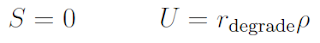 The diffusion coefficient, decay rate, and saturation density are all zero.
2: Copy the matlab visualization files: To help read and plot BioFVM data, we have provided matlab files. Copy all the *.m files from the matlab subdirectory to your project.
3: Copy the empty project: BioFVM Version 1.0.3 or later includes a template project and Makefile to make it easier to get started. Copy the Makefile and template_project.cpp file to your project. Rename template_project.cpp to something useful, like 2D_tumor_example.cpp.
4: Edit the makefile: Open a terminal window and browse to your project. Tailor the makefile to your new project:
> notepad++ Makefile
Change the PROGRAM_NAME to 2Dtumor.
Also, rename main to 2D_tumor_example throughout the Makefile.
Lastly, note that if you are using OSX, you'll probably need to change from "g++" to your installed compiler. See these tutorials.
5: Start adapting 2D_tumor_example.cpp: First, open 2D_tumor_example.cpp:
> notepad++ 2D_tumor_example.cpp
Just after the "using namespace BioFVM" section of the code, define useful globals. Here and throughout, new and/or modified code is in blue:
using namespace BioFVM:
// helpful -- have indices for each "species"
int live_cells = 0;
int blood_vessels = 1;
int oxygen = 2;
// some globals
double prolif_rate = 1.0 /24.0;
double death_rate = 1.0 / 6; //
double cell_motility = 50.0 / 365.25 / 24.0 ;
// 50 mm^2 / year --> mm^2 / hour
double o2_uptake_rate = 3.673 * 60.0; // 165 micron length scale
double vessel_degradation_rate = 1.0 / 2.0 / 24.0 ;
// 2 days to disrupt tissue
double max_cell_density = 1.0;
double o2_supply_rate = 10.0;
double o2_normoxic = 1.0;
double o2_hypoxic = 0.2;
6: Set up the microenvironment: Within main(), make sure we have the right number of substrates, and set them up:
// create a microenvironment, and set units
Microenvironment M;
M.name = "Tumor microenvironment";
M.time_units = "hr";
M.spatial_units = "mm";
M.mesh.units = M.spatial_units;
Notice how our earlier global definitions of "live_cells", "blood_vessels", and "oxygen" makes it easier to make sure we're referencing the correct substrates in lines like these.
7: Resize the domain and test: For this example (and so the code runs very quickly), we'll work in 2D in a 2 cm × 2 cm domain:
// set the mesh size
double dx = 0.05; // 50 microns
M.resize_space( 0.0 , 20.0 , 0, 20.0 , -dx/2.0, dx/2.0 , dx, dx, dx );
Notice that we use a tissue thickness of dx/2 to use the 3D code for a 2D simulation. Now, let's test:
> make
> 2Dtumor
Go ahead and cancel the simulation [Control]+C after a few seconds. You should see something like this:
Starting program ...
Microenvironment summary: Tumor microenvironment:
Mesh information:
type: uniform Cartesian
Domain: [0,20] mm x [0,20] mm x [-0.025,0.025] mm
resolution: dx = 0.05 mm
voxels: 160000
voxel faces: 0
volume: 20 cubic mm
Densities: (3 total)
live cells:
units: cells
diffusion coefficient: 0.00570386 mm^2 / hr
decay rate: 0 hr^-1
diffusion length scale: 75523.9 mm
blood vessels:
units: vessels/mm^2
diffusion coefficient: 0 mm^2 / hr
decay rate: 0 hr^-1
diffusion length scale: 0 mm
oxygen:
units: cells
diffusion coefficient: 6 mm^2 / hr
decay rate: 2.2038 hr^-1
diffusion length scale: 1.65002 mm
simulation time: 0 hr (100 hr max)
Using method diffusion_decay_solver__constant_coefficients_LOD_3D (implicit 3-D LOD with Thomas Algorithm) ...
simulation time: 10 hr (100 hr max)
simulation time: 20 hr (100 hr max)

t = i*12;
input_file = sprintf( 'output_%3.6f.mat', t );
output_file = sprintf( 'output_%3.6f.png', t );
M = read_microenvironment( input_file );
plot_microenvironment( M , labels );
print( gcf , '-dpng' , output_file );
end
What you'll need
- A working C++ development environment with support for OpenMP. See these prior tutorials if you need help.
- A download of BioFVM, available at http://BioFVM.MathCancer.org and http://BioFVM.sf.net. Use Version 1.0.3 or later.
- Matlab or Octave for visualization. Matlab might be available for free at your university. Octave is open source and available from a variety of sources.
Our modeling task
We will implement a basic 2-D model of tumor growth in a heterogeneous microenvironment, with inspiration by glioblastoma models by Kristin Swanson, Russell Rockne and others (e.g., this work), and continuum tumor growth models by Hermann Frieboes, John Lowengrub, and our own lab (e.g., this paper and this paper).We will model tumor growth driven by a growth substrate, where cells die when the growth substrate is insufficient. The tumor cells will have motility. A continuum blood vasculature will supply the growth substrate, but tumor cells can degrade this existing vasculature. We will revisit and extend this model from time to time in future tutorials.
Mathematical model
Taking inspiration from the groups mentioned above, we'll model a live cell density ρ of a relatively low-adhesion tumor cell species (e.g., glioblastoma multiforme). We'll assume that tumor cells move randomly towards regions of low cell density (modeled as diffusion with motility μ). We'll assume that that the net birth rate rBis proportional to the concentration of growth substrate σ, which is released by blood vasculature with density b. Tumor cells can degrade the tissue and hence this existing vasculature. Tumor cells die at rate rDwhen the growth substrate level is too low. We assume that the tumor cell density cannot exceed a max level ρmax. A model that includes these effects is:

Mapping the model onto BioFVM
BioFVM solves on a vector u of substrates. We'll set u = [ρ , b, σ ]. The code expects PDES of the general form:
Cell density
We first slightly rewrite the PDE:
 .
.Growth substrate
Similarly, by matching the PDE for σ term-by-term with the general form, we use:Blood vessels
Lastly, a term-by-term matching of the blood vessel equation gives the following functions:Implementation in BioFVM
1: Start a project: Create a new directory for your project (I'd recommend "BioFVM_2D_tumor"), and enter the directory. Place a copy of BioFVM (the zip file) into your directory. Unzip BioFVM, and copy BioFVM*.h, BioFVM*.cpp, and pugixml* files into that directory.2: Copy the matlab visualization files: To help read and plot BioFVM data, we have provided matlab files. Copy all the *.m files from the matlab subdirectory to your project.
3: Copy the empty project: BioFVM Version 1.0.3 or later includes a template project and Makefile to make it easier to get started. Copy the Makefile and template_project.cpp file to your project. Rename template_project.cpp to something useful, like 2D_tumor_example.cpp.
4: Edit the makefile: Open a terminal window and browse to your project. Tailor the makefile to your new project:
> notepad++ Makefile
Change the PROGRAM_NAME to 2Dtumor.
Also, rename main to 2D_tumor_example throughout the Makefile.
Lastly, note that if you are using OSX, you'll probably need to change from "g++" to your installed compiler. See these tutorials.
5: Start adapting 2D_tumor_example.cpp: First, open 2D_tumor_example.cpp:
> notepad++ 2D_tumor_example.cpp
Just after the "using namespace BioFVM" section of the code, define useful globals. Here and throughout, new and/or modified code is in blue:
using namespace BioFVM:
// helpful -- have indices for each "species"
int live_cells = 0;
int blood_vessels = 1;
int oxygen = 2;
// some globals
double prolif_rate = 1.0 /24.0;
double death_rate = 1.0 / 6; //
double cell_motility = 50.0 / 365.25 / 24.0 ;
// 50 mm^2 / year --> mm^2 / hour
double o2_uptake_rate = 3.673 * 60.0; // 165 micron length scale
double vessel_degradation_rate = 1.0 / 2.0 / 24.0 ;
// 2 days to disrupt tissue
double max_cell_density = 1.0;
double o2_supply_rate = 10.0;
double o2_normoxic = 1.0;
double o2_hypoxic = 0.2;
6: Set up the microenvironment: Within main(), make sure we have the right number of substrates, and set them up:
// create a microenvironment, and set units
Microenvironment M;
M.name = "Tumor microenvironment";
M.time_units = "hr";
M.spatial_units = "mm";
M.mesh.units = M.spatial_units;
// set up and add all the densities you plan
M.set_density( 0 , "live cells" , "cells" );
M.set_density( 0 , "live cells" , "cells" );
M.add_density( "blood vessels" , "vessels/mm^2" );
M.add_density( "oxygen" , "cells" );
M.add_density( "oxygen" , "cells" );
// set the properties of the diffusing substrates
M.diffusion_coefficients[live_cells] = cell_motility;
M.diffusion_coefficients[live_cells] = cell_motility;
M.diffusion_coefficients[blood_vessels] = 0;
M.diffusion_coefficients[oxygen] = 6.0;
// 1e5 microns^2/min in units mm^2 / hr
M.decay_rates[live_cells] = 0;
M.decay_rates[blood_vessels] = 0;
M.decay_rates[oxygen] = 0.01 * o2_uptake_rate;
// 1650 micron length scale
Notice how our earlier global definitions of "live_cells", "blood_vessels", and "oxygen" makes it easier to make sure we're referencing the correct substrates in lines like these.
7: Resize the domain and test: For this example (and so the code runs very quickly), we'll work in 2D in a 2 cm × 2 cm domain:
// set the mesh size
double dx = 0.05; // 50 microns
M.resize_space( 0.0 , 20.0 , 0, 20.0 , -dx/2.0, dx/2.0 , dx, dx, dx );
Notice that we use a tissue thickness of dx/2 to use the 3D code for a 2D simulation. Now, let's test:
> make
> 2Dtumor
Go ahead and cancel the simulation [Control]+C after a few seconds. You should see something like this:
Starting program ...
Microenvironment summary: Tumor microenvironment:
Mesh information:
type: uniform Cartesian
Domain: [0,20] mm x [0,20] mm x [-0.025,0.025] mm
resolution: dx = 0.05 mm
voxels: 160000
voxel faces: 0
volume: 20 cubic mm
Densities: (3 total)
live cells:
units: cells
diffusion coefficient: 0.00570386 mm^2 / hr
decay rate: 0 hr^-1
diffusion length scale: 75523.9 mm
blood vessels:
units: vessels/mm^2
diffusion coefficient: 0 mm^2 / hr
decay rate: 0 hr^-1
diffusion length scale: 0 mm
oxygen:
units: cells
diffusion coefficient: 6 mm^2 / hr
decay rate: 2.2038 hr^-1
diffusion length scale: 1.65002 mm
simulation time: 0 hr (100 hr max)
Using method diffusion_decay_solver__constant_coefficients_LOD_3D (implicit 3-D LOD with Thomas Algorithm) ...
simulation time: 10 hr (100 hr max)
simulation time: 20 hr (100 hr max)
8: Set up initial conditions: We're going to make a small central focus of tumor cells, and a "bumpy"field of blood vessels.
// set initial conditions
// use this syntax to create a zero vector of length 3
// std::vector<double> zero(3,0.0);
std::vector<double> center(3);
center[0] = M.mesh.x_coordinates[M.mesh.x_coordinates.size()-1] /2.0;
center[1] = M.mesh.y_coordinates[M.mesh.y_coordinates.size()-1] /2.0;
center[2] = 0;
double radius = 1.0;
std::vector<double> one( M.density_vector(0).size() , 1.0 );
double pi = 2.0 * asin( 1.0 );
// use this syntax for a parallelized loop over all the
// voxels in your mesh:
#pragma omp parallel for
for( int i=0; i < M.number_of_voxels() ; i++ )
{
std::vector<double> displacement = M.voxels(i).center - center;
double distance = norm( displacement );
if( distance < radius )
{
M.density_vector(i)[live_cells] = 0.1;
}
M.density_vector(i)[blood_vessels]= 0.5 + 0.5*cos(0.4* pi * M.voxels(i).center[0])*cos(0.3*pi *M.voxels(i).center[1]);
M.density_vector(i)[oxygen] = o2_normoxic;
}
9: Change to a 2D diffusion solver:
// set up the diffusion solver, sources and sinks
M.diffusion_decay_solver = diffusion_decay_solver__constant_coefficients_LOD_2D;
10: Set the simulation times: We'll simulate 10 days, with output every 12 hours.
double t = 0.0;
double t_max = 10.0 * 24.0; // 10 days
double dt = 0.1;
double output_interval = 12.0; // how often you save data
double next_output_time = t; // next time you save data
11: Set up the source function:
void supply_function( Microenvironment* microenvironment, int voxel_index, std::vector<double>* write_here )
{
// use this syntax to access the jth substrate write_here
// (*write_here)[j]
// use this syntax to access the jth substrate in voxel voxel_index of microenvironment:
// microenvironment->density_vector(voxel_index)[j]
static double temp1 = prolif_rate / ( o2_normoxic - o2_hypoxic );
(*write_here)[live_cells] =
microenvironment->density_vector(voxel_index)[oxygen];
(*write_here)[live_cells] -= o2_hypoxic;
if( (*write_here)[live_cells] < 0.0 )
{
(*write_here)[live_cells] = 0.0;
}
else
{
(*write_here)[live_cells] = temp1;
(*write_here)[live_cells] *=
microenvironment->density_vector(voxel_index)[live_cells];
}
(*write_here)[blood_vessels] = 0.0;
(*write_here)[oxygen] = o2_supply_rate;
(*write_here)[oxygen] *=
microenvironment->density_vector(voxel_index)[blood_vessels];
return;
}
Notice the use of the static internal variable temp1: the first time this function is called, it declares this helper variable (to save some multiplication operations down the road). The static variable is available to all subsequent calls of this function.
12: Set up the target function (substrate saturation densities):
void supply_target_function( Microenvironment* microenvironment, int voxel_index, std::vector<double>* write_here )
{
// use this syntax to access the jth substrate write_here
// (*write_here)[j]
// use this syntax to access the jth substrate in voxel voxel_index of microenvironment:
// microenvironment->density_vector(voxel_index)[j]
(*write_here)[live_cells] = max_cell_density;
(*write_here)[blood_vessels] = 1.0;
(*write_here)[oxygen] = o2_normoxic;
return;
}
13: Set up the uptake function:
void uptake_function( Microenvironment* microenvironment, int voxel_index, std::vector<double>* write_here )
{
// use this syntax to access the jth substrate write_here
// (*write_here)[j]
// use this syntax to access the jth substrate in voxel voxel_index of microenvironment:
// microenvironment->density_vector(voxel_index)[j]
(*write_here)[live_cells] = o2_hypoxic;
(*write_here)[live_cells] -=
microenvironment->density_vector(voxel_index)[oxygen];
if( (*write_here)[live_cells] < 0.0 )
{
(*write_here)[live_cells] = 0.0;
}
else
{
(*write_here)[live_cells] *= death_rate;
}
(*write_here)[oxygen] = o2_uptake_rate ;
(*write_here)[oxygen] *=
microenvironment->density_vector(voxel_index)[live_cells];
(*write_here)[blood_vessels] = vessel_degradation_rate ;
(*write_here)[blood_vessels] *=
microenvironment->density_vector(voxel_index)[live_cells];
return;
}
And that's it. The source should be ready to go!
Source files
You can download completed source for this example here:Using the code
Running the code
First, compile and run the code:
> make
> 2Dtumor
The output should look like this.
Starting program ...
Microenvironment summary: Tumor microenvironment:
Mesh information:
type: uniform Cartesian
Domain: [0,20] mm x [0,20] mm x [-0.025,0.025] mm
resolution: dx = 0.05 mm
voxels: 160000
voxel faces: 0
volume: 20 cubic mm
Densities: (3 total)
live cells:
units: cells
diffusion coefficient: 0.00570386 mm^2 / hr
decay rate: 0 hr^-1
diffusion length scale: 75523.9 mm
blood vessels:
units: vessels/mm^2
diffusion coefficient: 0 mm^2 / hr
decay rate: 0 hr^-1
diffusion length scale: 0 mm
oxygen:
units: cells
diffusion coefficient: 6 mm^2 / hr
decay rate: 2.2038 hr^-1
diffusion length scale: 1.65002 mm
simulation time: 0 hr (240 hr max)
Using method diffusion_decay_solver__constant_coefficients_LOD_2D (2D LOD with Thomas Algorithm) ...
simulation time: 12 hr (240 hr max)
simulation time: 24 hr (240 hr max)
simulation time: 36 hr (240 hr max)
simulation time: 48 hr (240 hr max)
simulation time: 60 hr (240 hr max)
simulation time: 72 hr (240 hr max)
simulation time: 84 hr (240 hr max)
simulation time: 96 hr (240 hr max)
simulation time: 108 hr (240 hr max)
simulation time: 120 hr (240 hr max)
simulation time: 132 hr (240 hr max)
simulation time: 144 hr (240 hr max)
simulation time: 156 hr (240 hr max)
simulation time: 168 hr (240 hr max)
simulation time: 180 hr (240 hr max)
simulation time: 192 hr (240 hr max)
simulation time: 204 hr (240 hr max)
simulation time: 216 hr (240 hr max)
simulation time: 228 hr (240 hr max)
simulation time: 240 hr (240 hr max)
Done!
Looking at the data
Now, let's pop it open in matlab (or octave):
> matlab
To load and plot a single time (e.g., the last tim)
!ls *.mat
M = read_microenvironment( 'output_240.000000.mat' );
plot_microenvironment( M );
To add some labels:
labels{1} = 'tumor cells';
labels{2} = 'blood vessel density';
labels{3} = 'growth substrate';
plot_microenvironment( M ,labels );
Your output should look a bit like this:

Lastly, you might want to script the code to create and save plots of all the times.
labels{1} = 'tumor cells';
labels{2} = 'blood vessel density';
labels{3} = 'growth substrate';
for i=0:20t = i*12;
input_file = sprintf( 'output_%3.6f.mat', t );
output_file = sprintf( 'output_%3.6f.png', t );
M = read_microenvironment( input_file );
plot_microenvironment( M , labels );
print( gcf , '-dpng' , output_file );
end
Tutorial series for BioFVM
Setting up your development environment
Using BioFVM
Subscribe to:
Posts (Atom)